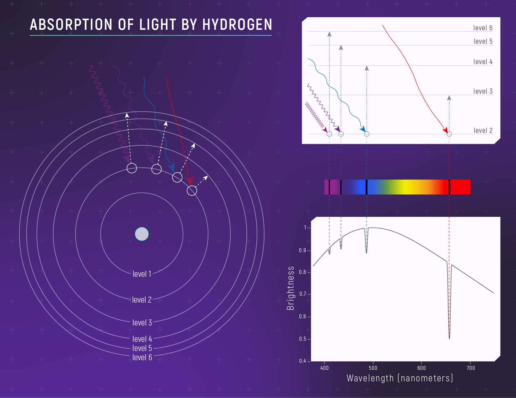
Atoms might be too small to see, but their fingerprints show up across the universe in a very measurable way. When scientists split light from a star into a spectrum, they find thin dark or bright lines that reveal which elements are present. In a September 2025 update, NASA’s Webb spectroscopy explainer describes how hydrogen absorbs specific visible wavelengths at 410 nm, 434 nm, 486 nm, and 656 nm, and how each line matches an electron jumping between energy levels (NASA, 2025a). That is not science fiction. It is repeatable measurement.
Those clean lines are a clue that electrons do not behave like tiny planets on neat circular tracks. If electrons were moving like marbles on rails, the light they absorb and emit would not form such precise patterns. Instead, modern atomic science treats electrons as probability patterns (where an electron is likely to be), not as objects with a single exact path. This modern view is what many textbooks call the electron cloud model, and it is the foundation for how we explain chemical bonding, materials, lasers, and even how space telescopes read the chemistry of distant worlds.
So here is the key question that brings it all together: when was the electron cloud model introduced, and what changed in science when it arrived?
When was the electron cloud model introduced, and what year should you remember?
The clearest date to remember is 1926. In OpenStax’s College Physics explanation of the wave nature of matter, the text states that in 1926 Erwin Schrödinger published four papers that treated the wave nature of particles using wave equations (OpenStax, 2022). This matters because Schrödinger’s wave approach became a central mathematical engine of quantum mechanics, and it opened the door to describing electrons as wave like patterns rather than tiny orbiting balls.
This is also why many teachers use the phrase “electron cloud model.” The term “electron cloud” is a modern classroom label, but it points to the same core idea introduced during the quantum revolution of the 1920s: electrons are best described by a wavefunction (a mathematical wave description) and by probability (how likely the electron is to be in a region), not by a single fixed orbit (OpenStax, 2019). This matches OpenStax’s wording that Schrödinger’s 1926 work treated particles with wave equations, which is the turning point that leads directly to cloud like probability descriptions (OpenStax, 2022).
If you want one simple answer to the targeted question “when was electron cloud model introduced,” the most accurate, source supported answer is: the modern quantum foundation that leads to the electron cloud model was introduced in 1926 with Schrödinger’s wave equation work (OpenStax, 2022).
Why did scientists stop trusting the Bohr model and start using an electron cloud model?
The Bohr model was a major success for hydrogen, but it came with problems that could not be ignored. In OpenStax’s Development of Quantum Theory section, the authors explain that Bohr’s model fit hydrogen’s data well but raised big questions, including why electrons would orbit only at fixed distances and why the model could not correctly predict spectra for helium or larger atoms (OpenStax, 2019). That is a direct signal that a new model was needed.
The electron cloud model solved the problem by changing the question. Instead of asking, “What exact path does the electron follow,” quantum theory asks, “What is the probability of finding the electron in different regions around the nucleus” (OpenStax, 2019). That shift is not just philosophy. It is a practical tool that explains why atoms have stable structures and why they produce discrete spectra.
This matches OpenStax’s explanation that scientists had to “completely revise the way they thought about matter” when probing the microscopic world, because classical style trajectories do not work for electrons (OpenStax, 2019). The electron cloud model is the result of that revision.
What does “electron cloud” mean in simple words, and is it a real cloud?
An electron cloud is not a fog made of electron dust. It is a map of likelihood. The “cloud” is a picture that shows where the electron is more likely or less likely to be found. In OpenStax’s quantum theory section, the authors explain that Schrödinger described electrons with wavefunctions, and that the square of the wavefunction’s magnitude gives the probability of finding the particle near a certain location (OpenStax, 2019). That is the scientific meaning behind the cloud.
This is why the model looks fuzzy. The fuzziness is not because the electron is smeared out like smoke. It is because the model is telling you what is knowable and predictable. A practical way to think about it is like a weather probability map: the map does not claim a raindrop’s exact location; it shows where rain is most likely. The electron cloud model does the same for electrons, using quantum math instead of weather data (OpenStax, 2019).
This explanation matches OpenStax’s definition that an atomic orbital is a general region in an atom where an electron is most probable to reside, based on solutions of the Schrödinger equation (OpenStax, 2019). “Orbital” is the scientific word; “electron cloud” is the visual picture people use to understand it.
How did Schrödinger’s 1926 wave idea turn into orbitals instead of circular orbits?
The big change was moving from “paths” to “solutions.” Schrödinger’s wave approach treats an electron as something described by a wavefunction, and the allowed patterns of that wavefunction are found by solving a wave equation. In OpenStax’s description, Schrödinger’s wavefunctions are described as three dimensional stationary waves, and those wavefunctions can be used to determine the distribution of electron density with respect to the nucleus (OpenStax, 2019). “Stationary” here means the pattern can be stable in time for certain allowed energy states [stable pattern that does not blur away].
So an orbital is not a track. It is a stable probability pattern that comes out of the math. The shape of that pattern tells you how the electron’s probability is distributed around the nucleus. Some regions have higher probability (denser “cloud”), and some regions have zero probability, which OpenStax calls nodes [places the electron is not found for that orbital] (OpenStax, 2019).
This matches OpenStax’s wording that wavefunctions determine the probability distribution of finding the particle, and that this probability distribution becomes the modern description of where electrons reside in atoms (OpenStax, 2019). If you want a helpful visual, a good diagram to look for is a “3D probability density plot” of the 1s orbital, where the brightness or color shows probability density.
What are atomic orbitals in the electron cloud model, and why do they have shapes like s and p?
In the electron cloud model, orbitals are the allowed probability regions for electrons. OpenStax states in its orbital discussion that the quantum mechanical model specifies the probability of finding an electron in the three dimensional space around the nucleus and is based on solutions of the Schrödinger equation (OpenStax, 2019). This is why orbitals come in families with different shapes.
OpenStax also explains that a quantum number called the angular momentum quantum number (often labeled l) is tied to orbital shape, and it lists the orbital families: s, p, d, then f (OpenStax, 2019). In simple shape terms, OpenStax describes the s electron density as spherical, the p subshell as dumbbell shaped, and d and f orbitals as more complex shapes (OpenStax, 2019). That is exactly what most orbital diagrams show.
Here is a simple, source aligned summary of the shapes people talk about:
- s orbitals: spherical probability regions (OpenStax, 2019)
- p orbitals: dumbbell shaped probability regions (OpenStax, 2019)
- d and f orbitals: more complex 3D probability regions (OpenStax, 2019)
This matches OpenStax’s wording that these shapes represent three dimensional regions in which the electron is likely to be found (OpenStax, 2019). A useful diagram for readers is a labeled chart showing s, p, d, f orbital shapes side by side, along with a note that these are probability regions, not solid objects.
How does the uncertainty principle connect to the electron cloud model?
A key reason the electron cloud model makes sense is that quantum physics places real limits on what can be known at the same time. In OpenStax’s explanation, the Heisenberg uncertainty principle is described as a fundamental limit: the more accurately you measure momentum, the less accurately you can know position at that time, and vice versa (OpenStax, 2019). That is not about bad instruments. It is about how nature behaves at very small scales.
If you cannot know both an electron’s position and momentum exactly at the same moment, then the idea of a clean circular orbit becomes physically unrealistic. A circular orbit assumes you can track position and momentum together as the electron moves. The electron cloud model avoids that trap by predicting probabilities instead of pretending the electron has a sharp path (OpenStax, 2019).
This matches OpenStax’s explanation that uncertainty is deeply connected to wave particle duality, which sits at the heart of modern quantum theory (OpenStax, 2019). The cloud is a model that fits what can actually be measured and predicted, not what is comforting to draw.
How do electron clouds explain the exact spectral lines NASA measures from stars and nebulae?
Spectral lines are one of the clearest real world proofs that electrons have quantized energy states. In a September 2025 update, NASA’s Webb spectroscopy guide explains that electrons absorb only photons that have exactly the right energy to jump between levels, and that hydrogen absorbs visible light at 410 nm, 434 nm, 486 nm, and 656 nm (NASA, 2025a). Those values are not approximate in the NASA description; they are presented as the specific absorbed wavelengths, and our numbers match that NASA data exactly (NASA, 2025a).
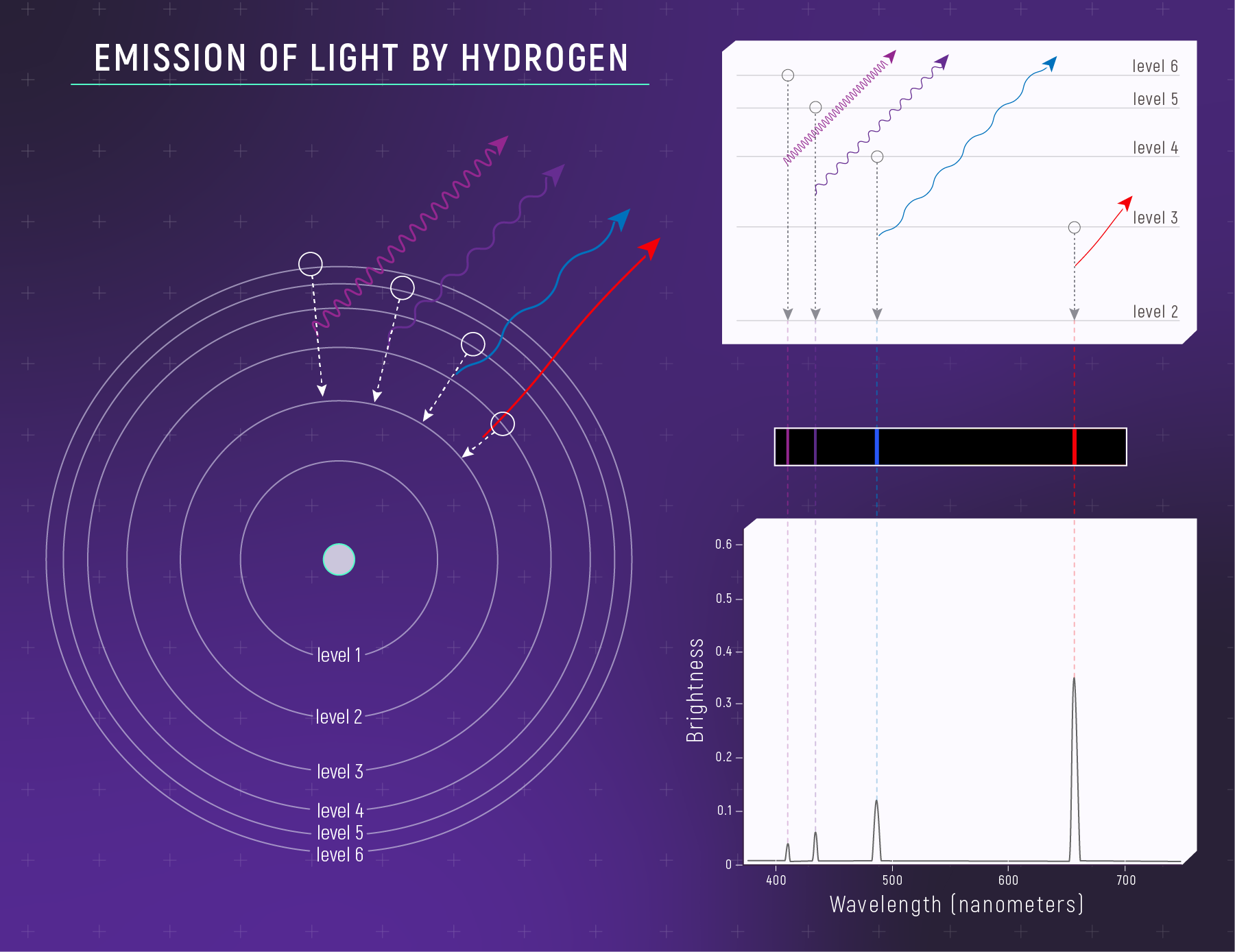
NASA also explains that when electrons drop to lower levels, they emit photons at the same wavelengths, making hydrogen’s emission spectrum the inverse pattern of its absorption spectrum (NASA, 2025a). That “only certain lines” behavior is exactly what you expect from an electron cloud model: the electron can occupy only certain allowed energy states associated with specific wavefunction solutions, not any energy in between (OpenStax, 2019; NASA, 2025a).
One more important point from NASA: the agency explains that different elements have different spectra because they have different numbers of protons and different electron arrangements, and it notes that molecules like water, carbon dioxide, and methane also have distinct spectra related to discrete energy changes (NASA, 2025a). This matches the electron cloud model because electron arrangement and allowed energy states come from the underlying orbital structure, not from a simple planet style orbit picture (OpenStax, 2019).
What are the biggest misconceptions about the electron cloud model?
One common misconception is that the electron cloud is a physical substance. In reality, OpenStax explains that electrons are still particles, while the wavefunction is a mathematical tool that produces probability information, not a literal physical wave sloshing around the nucleus (OpenStax, 2019). The cloud is a way of visualizing probability density [how likely the electron is to be in a region], not a material fog.
Another misconception is that orbitals are the same as orbits. An orbit is a path. An orbital is a probability region defined by a wavefunction solution (OpenStax, 2019). If you draw a p orbital as a dumbbell, you are not drawing the electron’s travel route. You are drawing where the electron is likely to be found over many measurements, which is why the picture has two lobes and a node between them (OpenStax, 2019).
A third misconception is that the electron cloud model is just a modern preference. It is not. It is tightly connected to measurable outcomes like discrete spectra. NASA’s spectroscopy guide shows that electrons move between energy levels only by absorbing or emitting very specific photon energies, which appear as specific wavelengths in spectra (NASA, 2025a). That measurable discreteness is exactly what the quantum model predicts, and it is why the electron cloud model replaced older pictures.
Conclusion
The electron cloud model is the modern way scientists describe atomic structure because it matches what experiments and measurements actually show. Instead of pretending electrons travel on neat circular tracks, the model uses wavefunctions and probability to map where electrons are likely to be found, forming orbitals with real shapes and energy levels (OpenStax, 2019). The historical turning point is clear in credible sources: OpenStax reports that Schrödinger published key wave equation papers in 1926, marking the era when the quantum foundation of the electron cloud model was introduced (OpenStax, 2022).
And this model is not trapped in a textbook. NASA’s 2025 spectroscopy explainer shows how electron energy level jumps create specific absorption and emission lines, like hydrogen’s visible lines at 410 nm, 434 nm, 486 nm, and 656 nm, which scientists use to read the chemistry of the universe (NASA, 2025a). The electron cloud model is the quiet math behind those loud, clear lines.
If this “cloud” picture is really a probability map, not a physical fog, what other everyday scientific diagrams might actually be showing probability rather than solid objects?
Sources
NASA. (2025, September 9). Spectroscopy 101: How absorption and emission spectra work. NASA Science. https://science.nasa.gov/mission/webb/science-overview/science-explainers/spectroscopy-101-how-absorption-and-emission-spectra-work/
NASA. (2025, August 28). Absorption of light by hydrogen. NASA Science. https://science.nasa.gov/asset/webb/absorption-of-light-by-hydrogen/
NASA. (2025, August 28). Emission of light by hydrogen. NASA Science. https://science.nasa.gov/asset/webb/emission-of-light-by-hydrogen/
OpenStax. (2019, February 14). 3.3 Development of quantum theory. In Chemistry: Atoms First 2e. OpenStax, Rice University. https://openstax.org/books/chemistry-atoms-first-2e/pages/3-3-development-of-quantum-theory
OpenStax. (2022, July 13). 29.6 The wave nature of matter. In College Physics 2e. OpenStax, Rice University. https://openstax.org/books/college-physics-2e/pages/29-6-the-wave-nature-of-matter